The sampling frame is defined as the collection of elementary sampling units that exist over the area to be surveyed. This area should be accurately defined with the survey objectives in mind. Examples of sampling areas are:
open lake water beyond the 20 m contour
bays and nearshore waters between the 10 and 30 m contours
An elementary sampling unit (ESU)is an object or area on which a measurement can be taken. In the case of acoustic estimates this may correspond, for example, to a transect or to a 500-m segment of a transect. The sampling frame is then the collection of all the possible non-overlapping transects. If we know the number of possible sampling units, we can make corrections to variance estimates for the finite sampling frame and thus reduce the variance. For most applications in the Great Lakes, the number of possible sampling units is so large that such corrections are not helpful.
Creating the sampling frame and identifying the ESU forces us to deal with issues of selection probability. Random sampling methods assume that each sampling unit has an equal probability of selection and therefore no sampling units should have a higher probability of being sampled than others. Although a logistically attractive design, zig-zag transects may over-sample certain areas and under-sample others, even if random starting positions are used. The identification of sampling frame and units is an important step also for geostatistical methods, for which a zig-zag design may be appropriate, to ensure unbiased and efficient estimates.
Consider the choice of whether to extrapolate density estimates to absolute abundance. The extra step of expanding a density per sampling unit (e.g., a transect) to total abundance in the sampling frame (e.g., the lake) may seem trivial, requiring only a scaling by area. But, total area is also an estimate that requires conscientious definition. Decisions must be made, such as:
Should we extrapolate based on area or volume?
Should embayments or deep-water areas be included?
How close to shore should we reasonably expect offshore fish to be?
These considerations question whether we know the area with 100% certainty, and whether the estimate of area should have an estimation error associated with it. Without absolute certainty, we place too much confidence in our area expansion. In most Great Lakes applications, the sampling frame can probably be estimated with high precision compared to the estimate of density.
The quality of fisheries acoustic surveys is typically evaluated by the variance of the estimate. We can control quality by reducing variance in two ways:
Sampling design: selection of sampling units to be included in the estimate, and;
Sample size: selection of the number of sampling units included in the estimate.
The choice of sampling design and sample size will depend on:
how and by how much the population varies, and;
how precise you wish the estimate to be.
The Catch-22 is that you don’t know how much a population varies until you sample it, but you can’t adequately design a survey until you know how much a population varies. A pilot, or exploratory, survey may be a useful means of determining the level of variation. Information from similar surveys conducted elsewhere may also help to answer this initial question.
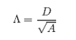
In designing a pilot or exploratory survey, a preliminary calculation of necessary sampling effort is degree of coverage (Aglen 1989). Degree of coverage (Λ) is defined as:
 |
|
[19] |
where:
D is the cruise track length, and;
A is the size of the survey area.
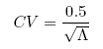
Errors associated with abundance estimates decrease as Λ increases. Aglen (1989) present an empirical relationships between the CV (SE/mean) and Λ as:
 |
|
[20] |
The predicted effect of using a particular design, sample size, and sampling allocation should be examined prior to conducting the survey. A calculation of the standard error of the estimate should be made using:
known population variance from a previous survey, or;
assumed population variance levels from a similar survey elsewhere.
Additionally, the standard error should be calculated under:
different survey designs;
different sample allocations (i.e., among strata), and;
different sample sizes.
Such calculations should indicate whether differences within 20% of current population levels will be detectable or whether only orders of magnitude change in abundance will be detectable.