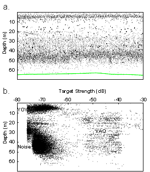
The simplest way to separate target and non-target species is to conduct a survey during a time (seasonal or diel) when the two groups are separated spatially. For example, young-of-year rainbow smelt have different thermal preference than yearling-and-older rainbow smelt and therefore separate spatially during temperature stratification in the summer (Fig. 30). Assessments in Lakes Ontario, Erie, Michigan, Huron, and Champlain take advantage of this separation by surveying in July to September.

Figure 30. Vertical separation of young-of-year and yearling-and-older rainbow smelt in Lake Champlain. Image taken from Parker Stetter et al. (2006).
In situ target strength
When individual fish can be resolved, in situ TS values can be obtained and used for calculating average backscattering cross sections to scale volume or area backscattering coefficients to fish density. When using in situ TS it is important to analyze the data in depth regions with homogeneous fish groups. This is because the sampling volume increases with depth, and fish in deeper water will therefore be over-represented in the data relative to their contribution to overall density. In many lakes, larger fish are found deeper and will be over-represented in a TS distribution derived from the whole water column.
The TS distribution can also be useful for separating age and size group. If a range of “acceptable” TS can be defined, values outside this range can be attributed to either large or small non-target organisms or noise. For example, yearling-and-older rainbow smelt in situ TS values fall between -60 and -35 dB (Parker Stetter et al. 2006). During June, values below -60 dB are from young-of-the-year rainbow smelt. During all times, values larger than -35 dB are from large piscivores (lake trout, etc.). In Lake Superior, targets > -35.6 dB are considered to be large (>250 mm) cisco (Yule et al. 2007). An alternative is to fit several theoretical distribution curves to the TS distribution to separate contributions from different species or age group (Rudstam et al. 1987, Warner et al. 2002). The contribution of alewife in Lake Ontario is calculated that way. With this method, it is important to be aware of the possibility of multiple peaks in the TS distributions from a single size group (observed for smelt – Rudstam et al. 2003, Parker Stetter et al. 2006). Parker Stetter et al. (2006) present a variant of this method for separating the contribution of young-of-year and yearling-and-older during period of spatial and TS range overlap in September. A similar approach for separating kokanee from large lake trout was proposed by Crockett et al. (2006). More work is needed to determine the appropriate functions to use for different species and age groups.
In situ methods are advantageous because:
they incorporate behaviors and vertical distributions observed during the survey.
A limitation to this approach is that fish have to be sufficiently dispersed to be observed as single targets.
A systematic change in fish orientation, for example, from a horizontal to a more vertical position during vertical migration, will cause a decrease in TS.
Great Lakes in situ TS ranges
Most Great Lakes surveys utilize in situ TS ranges to assist in the separation of species of interest. In many cases, vertical separation is also used. There is overlap of in situ TS ranges and they vary with season for young-of-year fish. TS ranges in Ontario, Erie and Champlain are different from Huron and Michigan because of differences in the timing of the surveys.
Lake Erie is the only lake to use defined in situ TS ranges. In addition, Lake Erie also vertically divides data into epilimnion, metalimnion, and hypolimnion. TS ranges currently applied in July surveys are:
young-of-year rainbow smelt: -70 to -59 dB
yearling-and-older rainbow smelt: -59 to -40 dB
Large fish, non-rainbow smelt: -40 to -20 dB
Lake Michigan and Huron use in situ targets between -76 and -20 dB, and use Warner et al. (2002, alewife) and Rudstam et al. (2003, rainbow smelt) to set the lower threshold. Trawl data is used for species and size composition.
Lake Ontario data are processed with a -64 dB in situ TS lower threshold, but densities are then pro-rated according to information in the TS histograms. Decisions are made individually for yearling-and-older rainbow smelt (hypolimnion, targets >-55 dB) and adult alewife (estimate targets belonging to a peak centered at approximately -39 dB)
Determining in situ TS ranges
In situ TS ranges are best determined by observing the target group of interest:
in the absence of other potential scatterers:
during normal activity (e.g., after diel vertical migration);
during the same month/season covered by the survey, and;
during the same diel period covered by the survey.
Validation
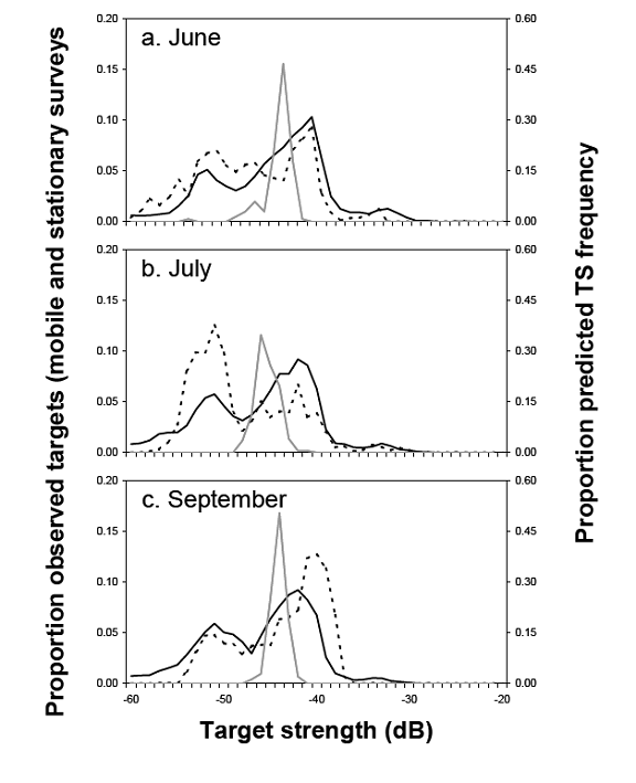
In situ TS ranges should be validated or compared with other techniques. Direct sampling (trawling, etc.) to identify species and length composition is essential. Repeated observation of TS ranges will ensure that the distribution is representative. Parker-Stetter et al. (2006) compared in situ results from mobile surveys, in situ measurements from stationary-tracked single fish, and predictions based on length-frequency in trawls (Fig. 31). Note the similarity in range and shape of the TS distributions between stationary- and mobile-survey estimates of TS. Also note that those distributions are both much wider than expected from calculations of mean TS from TS–L regressions and the length distribution in trawl catches.

Figure 31. Comparison of mobile survey (solid black), stationary survey (dashed black), and trawl capture (solid gray) estimates of TS for age-1 and older rainbow smelt in Lake Champlain during June, July, and September. The “trawl” target strength is calculated from the trawl catch and a TS–L regression (Parker Stetter el al. 2006).
Ex situ TS
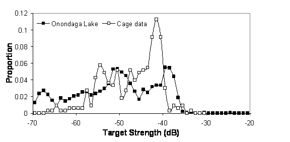
Ex situ measurements in acoustic surveys are controlled or semi-controlled experiments where individuals or groups of known sizes are insonified. Ex situ measurements are often done on fish of known species and size suspended in a large cage, or individuals that are anesthetized and insonified suspended in a frame. An example of a TS distribution derived ex situ for alewife in a large net cage compared to in situ TS distribution is presented in Fig. 32. Disadvantages to ex situ measurements are difficulties in replicating in situ conditions and uncertainty in applying ex situ measurements to survey conditions.

Figure 32. Alewife TS distribution from Onondaga Lake in spring 2005 dominated by one year class of alewife (age 3 – 150 mm, mean TS -42.8 dB) and from a large net cage (130 mm fish, mean TS -43.8 dB) at 70 kHz (summer 2005). From Rudstam et al. (in press – fish tech chapter)
Deriving ex situ TS values
Deriving regression for surveyed species is not trivial. A combination of in situ (if available) and ex situ measurements, and if possible, theoretical predictions of individual backscatter is ideal. Additionally, these equations are frequency dependent and should incorporate organism behavior and vertical distribution of target species encountered during the survey. The empirically derived regression is typically in the form:
 |
|
[27] |
where:
L is fish length (cm), and;
A is traditionally set equal to 20 (Foote 1987).
Ex situ TS equations are based on TS calculated from mean sbs. The equation does not represent the distribution of expected TS (see Fig. 31-32). The lower TS of interest in the analysis is substantially lower than the mean TS of the smallest fish of interest. Using a mean TS calculated from these equations to threshold data would result in the exclusion of target organisms that are located off their acoustic axis and/or happen to have a tilt angle resulting in smaller TS.
TS-length for Great Lakes species
TS-length relationships have been developed for several Great Lakes species (Table 11). Other similar species from the European literature are also included in Table 11. Given the variability observed among different investigators even for similar fish (e.g. the identical shaped European smelt (Osmerus eperlanus) and rainbow smelt (Osmerus mordax)), it is doubtful if the different species specific equations represents any improvement over using the standard Love equation (Table 11) equation as an indications of expected TS. Several authors have used the Love equation in the Great Lakes (Brandt et al. 1991, Goyke and Brandt 1993) and elsewhere (Burcynski and Johnson 1986, Guillard and Gerdeaux 1993, Parkinson et al. 1994, Mason et al. 2001, Rudstam et al. 2002, Frouzova et al. 2005, Crockett et al. 2006). Note that the equations for smelt and bloater presented by Fleischer et al. (1997) are very different for small and large fish compared to all other measures, but similar in the middle of the range of fish investigated. We believe the differences is due to the relatively large variance in the Fleischer et al. (1997) data set, and that the Fleischer et al. (1997) equations should only be used for estimates in the middle of the range of fish sizes they investigated. However, more work is needed before discounting these equations as the correspondence between trawl sizes and TS from the Fleischer et al. (1997) equation are reasonable for Lake Superior (Mason et al. 2005, Yule et al. 2006).
Table 11. Empirical target-strength relationships for Great Lakes species. L is length in cm and w is weight in g. This table should be updated to include studies from other areas of the same species groups, including European smelt and coregonids.
Species |
Relationship |
Frequency (kHz) |
TS of a 20 cm or 50 g fish (dB) |
Source |
Many species |
TS = 19.2 log10(L)+0.9 log10 (λ)-62.3 |
|
-39.01 |
Love 1971, Brandt et al. 1991 |
Rainbow smelt and alewife |
TS = 18.2•log10(L)-67.5 |
120 |
-43.8 |
Argyle 1992 |
Rainbow smelt |
TS = 19.9•log10(L)-67.8 |
120, 70 |
-41.9 |
Rudstam et al. 2003 |
Smelt, alewife |
TS = 52.6•log10(L)-100.2 |
120 |
-31.6 |
Fleischer et al. 1997 |
Cisco |
TS = 21.9•log10(L)-67.2 |
70 |
-38.7 |
Rudstam et al. 1987 |
Bloater |
TS = 52.6 log10(L)-106.5 |
120 |
-38.0 |
Fleischer et al. 1997 |
Alewife |
TS = 20.53•log10(L)-64.25 |
70 |
-36.9 |
Warner et al. 2002 |
Lake Trout |
TS = 20 log10(L)-65.3 |
120 |
-39.3 |
Middel 2005 |
European smelt |
TS = 23.4•log10(L)-68.7 |
120 |
-38.1 |
Peltonen et al. 2006 |
Coregonus albula |
TS = 25.5•log10(L)-70.9 |
120 |
-37.7 |
Mehner 2006 |
Baltic herring |
TS = 16.8•log10(L)-60.0 |
38 |
-38.1 |
Peltonen and Balk 2005 |
Baltic herring |
TS = 25.5•log10(L)-73.6 |
38 and 70 |
-40.4 |
Didrikas and Hansson 2004 |
Alewife |
TS = 6.98•log10(W)-50.07 |
70 |
-38.2 |
Warner et al. 2002 |
Smelt, alewife |
TS = 15.2•log10(W)-60.24 |
120 |
-34.4 |
Fleischer et al. 1997 |
Bloater |
TS = 15.2•log10(W)-65.54 |
120 |
-39.7 |
Fleischer et al. 1997 |
Omul Coregonus autumnalis migratorius |
TS = 20 •log10(L)-64.24
|
70
|
-38.22 |
Goncharov et al. 2008 |
1) Evaluated for 120kHz
TS model values
Numerical and analytical models have been developed to predict acoustic backscatter as a function of organism size, shape, anatomical characteristics, orientation, and acoustic frequency for zooplankton and fish. The models range in complexity from approximating organism anatomy and morphometry as simple shapes, to utilizing three-dimensional digital images of organism internal structures (Horne and Jech 2005).
Theoretical models have advantages and limitations when applied to different organism types. An advantage of TS models is:
once verified, predictions may be made over a wide range of conditions (i.e., acoustic frequency, behavior, biological state).
Difficulties with applying models to survey data are:
obtaining accurate representations of in situ organism anatomy, morphometry, orientation, and;
verifying the predictions.
Models may be used to provide mean or minimum expected TS for Sv threshold calculations. Caveats on these two approaches are discussed under in situ TS above.
In marine systems, groups of interest are often analytically separated based on trawl catches and known relationships between fish lengths and σbs. The main assumptions made by this approach are
trawl bias is minimal or understood, and;
the TS – L regression used is valid for the survey conditions
Two ways to reduce biases introduced by this approach are:
by using only in systems where the fish community is well understood from past sampling;
by sampling with a closing net to reduce contamination during haul-back
Acoustical backscatter by organisms with a gas-bearing structure such as a swimbladder is significantly greater than for organisms without a gas-bearing structure. This attribute can be used to reduce or eliminate the Sv from non-gas-bearing organisms by setting an Svthreshold.
No setting can discriminate between fish and plankton or other non-target species with 100% accuracy. Some small fish targets are unavoidably discarded, just as some small amount of acoustic return from unwanted sources is included. The goal in choosing an Sv threshold setting is to find an optimal balance between eliminating non-target species Sv and preserving the target species Sv (NMFS SOP). Because some error is involved in applying a threshold, it is important to maintain consistency between surveys, i.e., the data collection threshold choices should be the same for all surveys in a time series (NMFS SOP).
Consider this example. The minimum TS of a fish of interest is determined to be -60 dB from observations of in situ TS distributions. A -60 dB target would be recorded as -66 dB in the TSu variable if located in the direction of the half intensity beam angle (-3 dB in both directions = -6 dB). A reasonable compromise is therefore to exclude volume backscattering from targets with an echo level smaller than -66 dB (in the TSu variable). The corresponding threshold in the Sv variable change with depth due to the different TVG functions applied to the Sv and TSu data and the correct Sv threshold for each depth can be calculated from equation 24 (Fig. 33). Note that this Sv threshold is range dependent. In practice this is done by setting this threshold in the Amp echogram representing 40 log R data and integrating on this echogram (Sonar5) or by setting the appropriate TS based threshold in the Sv echogram (EV 4.4).

Figure 33. Decreasing Sv threshold over depth for a 120 kHz transducer with EBA of -20 dB, sound speed 1450 m•s-1 and pulse duration of 0.4 ms that correspond to a TSu threshold of -66 dB (see text).
Finding the lower limit of the TS distribution of the smallest fish of interest is the key component of settings appropriate thresholds in the Sv domain. This minimum TS may be based on in situ TS distributions, ex situ TS distributions, or theoretical models. Thresholds should not be found be converting the length of the smallest fish of interest to TS using a TS-L equation as in Table 11. The TS distribution of any fish is relatively wide, and using mean TS to base a threshold would in principle remove half the echoes from those fish. After this minimum TS value is selected, follow the above procedure to calculate a depth varying Sv threshold.
Frequency differencing
Multifrequency approaches are in their infancy in the Great Lakes. Combined analysis of several frequencies could help differentiating fish from mysids. Such approaches are common in marine systems (e.g., Cochrane et al. 1990. Swartzman et al. 2001). A lower frequency than 120 kHz could be particularly useful and Rudstam et al. (2008) have found that 38 kHz give both higher TS of alewife and lower TS of mysids in Cayuga Lake. More frequencies can also help in single fish detections (Demer et al. 1999).
Decomposition of the TS distribution
Separation of age groups or species from the TS distribution is difficult because of the large range of TS expected from each length group. There is considerable overlap even between young-of-year and adult fish. Parker Stetter et al. (2006) presented a method for separating age groups of rainbow smelt in Lake Champlain based on measurements of the expected TS distribution from the two age groups. However, we do not at present have a good estimate of the additional error added by this method to the estimate of the two age groups. Crockett et al. (2006) presented a similar method for separating large lake trout from kokanee targets and Brooking and Rudstam (in review) used the expected TS distribution from YOY and adult alewife measured in net cages to obtain age specific density estimates from field TS distributions.
Mysids and zooplankton
Mysids and possibly smaller zooplankton could contribute substantially to Sv values in deeper waters without appropriate thresholds. The thresholds can also be reversed allowing for acoustic estimates of mysids by removing fish echoes. This has been applied successfully to Lake Ontario (Rudstam et al. 2008b). The use of acoustics for zooplankton estimates has also been done in Lake Superior (Megard et al. 1997, Holbrook et al. 2006). We need to further test and potentially modify these methods for the other Great Lakes.