Depending on the analysis to be used, data files may be created to contain:
single transects;
strata, or;
entire survey.
An analysis using transects as sampling units might benefit from keeping them separated during processing. Additionally, smaller, time- or location-referenced files make identifying specific sections of surveys easier. The components of an individual data file should also be chosen with file size in mind – some post-processing packages experience considerable slow-down with increasing file size. If slow-down is not a problem, it is straightforward to define each transect as a separate region in a file within the whole survey.
All system and collection settings must be input to each data file or a file template. Use the note fields to add comments and information on the surveys. Calibration and environmental settings are entered in calibration tabs for each variable (also check derived variables) and for the transducer. In Echoview and Sonar5, calibration parameters are obtained directly from the data string for some echosounders. Typical calibration settings include gains (TS and Sv), equivalent beam angle, beam width, beam offset, # samples per meter.
Table 8. Calibration and environmental settings needed in Echoview for different echosounders used in the Great Lakes. Sv is the Sv variable, TSu – TSu variable, Ang – Angular position variable, SED – Single echo detection variable, Trans – Transducer variable.
Attribute |
Simrad EY500 |
Simrad EK60 |
Biosonics DTX |
Transducer beam width (3 dB angle) |
Trans |
Trans |
Trans |
Transducer depth |
Trans |
Trans |
Trans |
Sound speed |
Sv, TSu, SED |
Ang, Sv, TSu, SED |
Ang, Sv, TSu, SED |
Minor axis offset |
Ang |
Ang |
|
Major axis offset |
Ang |
Ang |
|
Angle sensitivity (minor/major) |
Ang |
|
|
Sample resolution |
Ang, Sv, TSu |
|
|
Absorption coefficient |
Sv, TSu |
Sv, TSu |
Sv, TSu |
Transmitted power |
Sv, TSu |
Sv, TSu |
|
Calibration offset1 or Transducer gain (Sv and TSu)2 |
Sv, TSu |
Sv, TSu |
Sv, TSu |
Sa correction |
|
Sv |
|
Pulse length |
Sv, TSu, SED |
Sv, TSu, SED |
Sv, SED |
Frequency |
Sv |
Sv, TSu |
Sv, TSu |
Two way beam angle (EBA) |
Sv, SED |
Sv, SED |
Sv |
Wavelength |
Sv |
|
|
Apply TVG range correction |
|
Sv, TSu |
|
1Biosonics terminology, 2Simrad terminology
Calculate average sound speed and absorption coefficient given the depth of the fish of interest. A calculator is available in most software, but temperature (and salinity) is provided by the user. If all fish are found in water shallower than 30 m, use average temperature in the top 30 m. Alternatively, a measured temperature gradient can be entered to change sound speed and alpha dynamically with range (Sonar5). Sound speed must be set to the same value in all analysis variables (echograms), or else the data will not align properly (EchoView).
If settings changed during the survey, be sure to make these changes in the post-processing data file. You need to make separate files for sections with different settings, except for ping rate. Variable ping rate is not a large problem in the analysis. Decisions on whether to keep sound speed and absorption values consistent for the survey or to vary with location (if sampling over a large area or one with very different values) are necessary at this stage of the analysis.
Selection of a surface exclusion zone should take into account:
extent of the near-surface deadzone including the near-field of the transducer.
surface conditions due to weather
vertical distribution of species or group(s) of interest
The purpose of the surface exclusion zone is to remove unreliable data while maintaining information about the survey targets. In the case of surface conditions, it is advisable to apply noise removal (see Noise removal below) and/or biological thresholds (see Isolating groups of interest below) before selecting a surface exclusion zone as restrictions may remove or reduce the effect of bubbles on the data.
Echosounders and post-processing software use algorithms to detect the seabed. Depending on bottom type and topography, performance of these algorithms varies. On hard, flat substrate, the algorithms perform well. On soft substrate, or rugged topography, the ability to accurately detect the bottom degrades. Echo strength from the seabed is typically orders of magnitude greater than the echo strength from biological organisms, thus eliminating seabed echoes from the water column data is imperative.
Improper bottom detections are found and corrected manually through inspection of the echograms our through automated algorithms. Failure to verify bottom detection could result in increased Sv values due to bottom inclusion. Bottom detection can also exclude echoes from dense fish schools. Detailed pixel-by-pixel check of the bottom definition is possible in the software.
The bottom exclusion zone is selected to remove data within the near-bottom deadzone. (Deadzone Height Example.) Effectively, this approach also removes data from targets located near the bottom. Although Ona and Mitson (1996) propose extrapolating integration and TS values from the region immediately above the dead zone into the volume represented by the deadzone itself, this approach is not without bias (Simmonds and MacLennan 2005).
For that reason, if targets near the bottom are of interest, it is advisable to acknowledge the bias that is introduce by the bottom exclusion zone and only proceed with a correction factor if the nature of near-bottom distribution is well known.
Discrete spikes in the data, resulting from electrical or acoustic interference or trawl noise, may be removed manually (Fig. 27). By doing so, data within the exclusion box is removed from analyses. Note that the assumption about fish density in bad data regions is important if these regions are large. Two options are currently available. A) To exclude bad data regions – similar to areas below the bottom. This will result in correct average Sv values but Sa values will be biased low. B) To assume bad data regions have 0 acoustic scattering. This will lead to both Sv and Sa values being biased low. The amount of bias depends on the size of the bad data region. The assumption that bad data regions have the same fish density as the surrounding water is not implemented directly in either software but can be calculated from the exported Sv data if the size of the analysis cell is known (export cell height while including bad data regions in EchoView and use that height to calculated Sa values from the measured Sv).
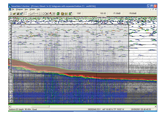
Figure 27. Noise produced during trawl deployment detected on 70 kHz echosounder. Such noise may be manually classified as “bad” data or erased in post-processing programs, but underlying data are lost.
There is always ambient noise that is amplified by the TVG function and therefore appear to increase with depth. This noise
is additive to the signal and can be removed with a threshold or by subtraction. A threshold removes noise by only accepting echoes larger than the threshold. This method will not account for noise added to the accepted signal. As long as the signal is an order of magnitude higher than the noise, this should not be a problem. But if data with smaller SNR is to be used, then subtraction is the best approach (Watkins and Brierley 1996, Korneliussen 2000).
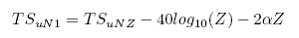
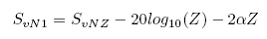
To remove ambient noise, measure sv values in an area where only noise is expected. One such area is below the bottom signal or in deep water (depending on the lake). Remember the noise levels at 1 m are different for TSu and Sv variables (Equation [24], also below). Noise levels at any depth, including at 1 m, can be calculated from a measure of noise at a given depth (Equation [25]and [26]) or directly from data collected in passive mode. Subtraction of noise in Echoview is done calculating the noise sv values for each analysis cell given the measured noise level at 1m, exporting these values and subtracting them from the data. Sonar5 calculates average noise levels from a user defined region in any echogram (active or passive) and provide a plot of noise for all depth layers. This depth dependent noise level can then be subtracted from any echogram.
Noise levels at 1m (TSuN1 in TS domain and SvN1 in Sv domain) can be calculated from the following equations.
| |
 |
[25] |
| |
 |
[26] |
And from equation (24) TSuNZ = SvNZ + 10 log10 (V)
where V = cτψ R2/2 and TSuNZ and SvNZ are the noise levels in dB measured at range R in the TS and Sv domains, respectively.
Alternatively, the noise level can be obtained from measurement at many depths by minimizing the difference between a theoretical curve (from above equation) and several noise measurements. This can be done with non-linear estimation in any statistical package, including Excel’s solver routine.